DSixOutputConverter - Manual

Output files can be written either as ASCII-files or as binary files. The latter tend to be a bit smaller, yet cannot be compressed as good as ASCII-files. Accessing large data sets in binary format is usally much more efficient than parsing ASCII-files, so whenever large 2D or 3D data sets are to be processed, the binary format is recommended.

There are two different file types:

The files have specific extensions:

Data files generally hold transient data (date for each output time point). Output time point frequency can vary among data files, even from the same project (e.g. longer intervals for large fields, smaller intervals for integral values).

Data files for 3D, 4D and 5D datasets require the geometry file to be present. 2D data files (i.e. time series of scalar values) do not require geometry files.

The purpose of the DSixOutputConverter converter tool is to automate specific conversion operations, that require otherwise manually written scripts or very laborious manual copy+paste work.

Here are some of the things, you can do with the tool:

Shows a summary of the data format and content of a data file.

Syntax:

Example:

gives:

With minimal verbosity level:

the output is:

which can be easily parsed by a script or just help to check the contents of a file.

Reads a data file (either in binary or ASCII-format) and writes it in ASCII format (possibly applying data transformation operations). A typical use of the operation is the conversion from binary to ASCII format.

Example command line:

with output:

The operation has generated files profile-temperature-x.d6o and LShape_3706993807.g6a.

You can apply data transformation flags to this operation.

Reads a data file (either in binary or ASCII-format) and writes it in binary format (possibly applying data transformation operations). A typical use of the operation is the conversion from ASCII to binary format.

The operation is otherwise identical to the ascii command.

Reads a data file (and its geometry file), and exports a data file in format suitable for the TECPLOT post-processing software. You may need to specify additional arguments depending on the type of data file you want to generate.

You can apply data transformation flags to this operation.

The conversion into a Tecplot format is depending on the data format of the file:

Reads data file and exports it in generic format. generic format means to write data in plain text format, so that it can be easily imported in other software.

The output format is further determined by the flags: --csv, --tsv and --block, as described below.

TODO

With this command, the difference between two data files can be computed.

Example syntax:

The values of the second file are subtracted from the first. Data format and type of the files stays the same.

Very simple transformation. Multiplies all values by the given factor. Useful for inverting the sign of flux outputs.

Example command line:

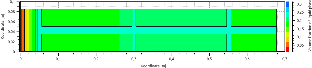
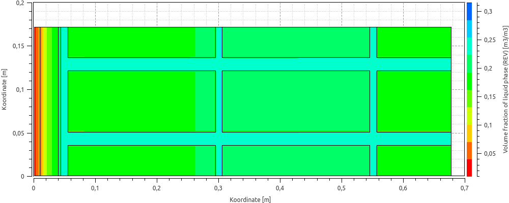
Especially with 2D and 3D simulations it is frequently possible to use symmetry properties of the model and thus reduce the size of the calculation domain. For example, the following simulation model

can be replaced (exploiting symmetry) by:

The difference in simulation time (26 s for 2108 elements compared to 4:30 min for 14964 elements, for 30 d simulation time, each) is remarkable.

For the presentation of the calculation results in a report, however, a full view of the construction and results is often helpful. In the shown example, the brick/plaster geoemtry pattern would otherwise not be apparent.

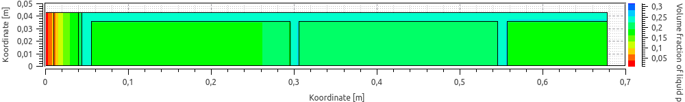
With the --mirror data transformation operation it is possible to mirror the construction geometry to the left (xl), to the right (xr), to the top (yt) and to the bottom (yb). The transformation is applied to the geometry and to the complete data set (all time points).

Example for the command line:

As explained above, the operation bin means "write in binary format". The argument --mirror=yt tells the converter to place the mirror axis to the top of the construction. And --output specifies the resulting file name.

Another data transformation can be used to mirror again at the top axis:

resulting in the final output:

DataIO files contain data sets for different time points. These time points are numbered, starting with index 0 for the first time point.

Suppose an output file contains the following data lines:

The first column holds the time point of the data set, in the unit specified in the header. In this example this is d (days). The simulation output time range spans 0 to 2 days, with a total of 11 time points.

You can now extract a subset of the data using the option --timeindex (and the other options described hereafter).

--timeindex takes either one or two arguments:

Example syntax:

If the command above is applied to the Example DataIO data file the following output is generated:

The lines with index 5, 6 and 7 are kept (corresponding to time points 1, 1.2 and 1.4 d).

Using the -l or --last flag, only the last data set for the last time point is kept.

This is a convenience function and equivalent to specifying --timeindex=11 in the example Example DataIO data file (passing the index of the last time point).

This function is similar to the variant with --timeindex and giving only one index argument. It extracts a single data line.

The function determines the dataset and time point closest to the given time and, if there is no exact match, interpolated linearly between values. If the following command line is used on Example DataIO data file:

The following output is created:

which is the interpolated value between the original data lines:

If the time point is larger than the last time point, an error is generated, for example when passing --time=4 as argument:

This time slicing data transformation extracts a subset of data points between the given time points. Here, the range of datasets is delimited by time points.

Example syntax:

All data sets with time points within the range (limits including) are kept. Applied to Example DataIO data file this gives: