This manual is available as:
Software is available at: https://bauklimatik-dresden.de/mastersim
1. Introduction and basic concepts
MasterSim is a co-simulation master program that supports FMI co-simulation. If you are new to co-simulation in general, or not yet familiar with the Functional Mock-Up Interface (FMI), I suggest reading up a bit on the basics on the fmi-standard.org webpage.
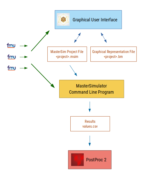
Basically, MasterSim couples different simulation models and exchanges data between simulation slaves at runtime. The following Figure illustrates the program organisation and the basic data flow.
1.1. Program parts
MasterSim consists of a two parts:
-
graphical user interface (GUI) and
-
a command line simulator program MasterSimulator
The GUI makes it very easy to generate, adjust, modify simulation projects. A simulation project is stored in two files, the MasterSim project file and the graphical representation file. The latter is optional and not needed for the simulation.
The simulation is executed by the command line program MasterSimulator, which reads the project file, imports referenced FMUs and run the simulation. The generated results, both from MasterSimulator itself and possibly from slaves are then used by any post processing tool (like PostProc 2) to visualize and analize results.
The separation between user interface and actual simulator makes it very easy to use MasterSim in a scripted environment, or for systematic variant analysis as described below in section Workflows.
1.2. Supported FMU types
-
FMI for Co-Simulation version 1
-
FMI for Co-Simulation version 2, including support for getting/setting states
No asynchronous FMU types supported.
On Linux and MacOS MasterSim is typically only built as 64-bit application. On Windows, MasterSim is available as 32-bit and 64-bit application.
|
For 32-bit FMUs use a 32-bit build, for 64-bit FMUs use a 64-Bit version. Mixed FMU platform types (32-Bit and 64-Bit) are not supported. |
1.3. Design criteria/key features
-
cross-platform: Windows, MacOS, Linux
-
no dependency on externally installed libraries, all sources included in repository (exception: standard C++, and the Qt 5 libraries), especially no dependency on FMI support libraries; checking out source code and building it should be easy (also packaging for different platforms)
-
complete master functionality wrapped in library MasterSim usable by command line tools and GUI applications
-
message handling wrapped to support GUI integration and log file support, no direct
printf()orstd::coutstatements -
supports FMU debugging: can disable unzipping (persistent dll/so/dylib files), source access allows debugging runtime loading of shared libraries and attaching debuggers
-
high-level C++ code (readable and maintainable)
-
includes instrumentation to retrieve counters and timers for benchmarking performance of master algorithms and FMUs
-
code tailored for master algorithm debugging - all variables in type-specific arrays for easy analysis in debugger
See chapter Features assisting in FMU development and debugging for details about functionality that are particularly important for FMU developers and for debugging problems with the co-simulation.
1.3.1. Special features of MasterSim
There is one specific feature of MasterSim that is helpful for using FMUs that write their own output data. To provide a writable, slave-specific output directory to each slave, MasterSim sets the parameter ResultsRootDir (typically with value reference 42) in each slave to this directory. As long as a slave defines such a parameter, the FMU code can rely on getting a valid directory to write its data into. See also section Directory slaves.
1.4. Terminology
The following terms are used in the manual and also in the naming of classes/variables:
| FMU |
describes the fmu archive including model description and shared libraries |
| slave/simulator |
describes a simulation model that is instantiated/created from an FMU; there can be several slaves instantiated by a single FMU, if the capability canBeInstantiatedOnlyOncePerProcess is set to false |
| master |
describes the overall simulation control framework that does all the administrative work |
| simulation scenario |
defines a set of slaves and their connections (data exchange), as well as other properties such as start and end time, algorithm options, output settings; alternatively called system |
| graph network |
another description for the topology of interconnected slaves |
| master algorithm |
describes the implementation of a mathematical algorithms that advances the coupled simulation in time; may include an iteration scheme |
| error control |
means local error check (step-by-step based), used for time step adjustment scheme |
| master time |
time of master simulation, starts with 0; unit is not strictly defined (needs to be common agreement between FMUs, typically in seconds, with exception of using file reader slaves, see section CSV FileReader Slaves). |
| current (master) time |
the time that the master state is at, changes only at end of successful |
1.5. Workflows
As with any other simulation models, most workflows involve a variant analysis. In the context of co-simulation, such variants are often created by modifying FMUs and their paramters. MasterSim includes functionality to streamline such workflows.
|
Many workflows involve repeated execution of MasterSim with little or no modifications in the project file. Sometimes it is very convenient to use the same project file and modify it, but specify a different working directory (where outputs are stored), so that the results of different variants can be compared |
1.5.1. Initial setup of a simulation scenario
This is a straight-forward procedure:
-
import all FMUs and assign slave ID names
-
(optional) specify parameter values for slaves
-
(optional) define graphical representation of slaves
-
connect output and input variables
-
set simulation parameters
-
run simulation
-
inspect results
1.5.2. Only published parameters of FMUs are modified
Extremely simple case and, if supported by FMUs, definitely best-practice. In MasterSim only the value assigned to a published parameter needs to be changed (can be done also directly in the project file, e.g. with scripts) and the simulation can be repeated.
1.5.3. FMUs change internal behavior, but do not change interface
This is the most typical case. Here, the input and output variable names and types remain unchanged and also the published parameters remain the same. Yet, the internal behavior of the model changes due to adjustment of internal model behavior, after which the FMU is exported again. Since MasterSim only references FMUs, in such cases the FMU files can simply be replaced and without any further changes the simulator can be started.
1.5.4. FMUs change parameters, but do not change inputs/outputs
In this situation, when a parameter has been configured in MasterSim that no longer exists (or has been renamed), the respective definition must be changed in the project file or be removed in the user interface.
1.5.5. FMUs change interface
When an imported FMU changes part of its interface (e.g. input or output variables are modified), then this will be shown in the user interface by highlighting invalid connections. If only variable names were changed, you are best of by editing the project file and renaming the variable name there. Otherwise, simply remove the connection and reconnect.
When the variable type changes of an input/output variable, so that an invalid connection is created (or the causality changes), then the user interface may not directly show the invalid connection. However, during initialization, the MasterSimulator command line program will flag that error and abort.
1.6. Simulation algorithm overview
MasterSim has the following main building blocks:
-
initialization (reading project file, extracting FMUs, checking…)
-
initial conditions
-
time step adjustment loop
-
master algorithm (i.e. attempt to take a step)
-
error checking
-
output writing when scheduled
These building blocks are described below in more detail.
1.7. Initialization
Upon start of the actual simulation (the command line program MasterSimulator, see section Command line arguments for details on running the program), the working directory structure is being created and the log file writing is started.
Then, the project file is read and all referenced FMUs are extracted. If CSV files are referenced (see section CSV FileReader Slaves), these files are parsed and prepared for calculation.
Extraction of FMU archives can be skipped with the command line option --skip-unzip (see section Modifying/fixing FMU content).
|
As first step of the actual co-sim initialzation all the FMU slaves are being instantiated (dynamic libraries are loaded and symbols are imported, afterwards fmiInstantiateSlave() or fmi2Instantiate() are called for FMI 1.0 and FMI 2.0 slaves, respectively). This is followed by a collection of all exchange variables and creation of the variable mappings.
Any error encountered during the initialization results in an abort of the simulator.
1.7.1. Initial conditions
The first task of the simulator is to get all slaves to have consistent initial values. This is already a non-trivial task and not guaranteed to succeed in all cases. The only procedure that can be employed for FMI 1 and FMI 2 slaves is to iteratively get and set output and input variables in all slaves in an iterative manner, until no changes are observed.
The algorithm in MasterSim is:
loop over all slaves:
  - call setupExperiment() in current slave
  - set all variables of causality INPUT or PARAMETER to their
    default values as given in the modelDescription.xml
  - set all parameters to the value specified in the project file (if values are assigned)

for FMI 2: tell all slaves to enterInitializationMode()

loop with 3 iterations:
  loop over all slaves:
    get all outputs from current slave and store in global variable mapping
  loop over all slaves:
    set all input variables with values from global variable mapping

for FMI 2: tell all slaves to exitInitializationMode()
Note, the initial calculation algorithm is actually a Gauss-Jacobi algorithm, and as such not overly stable or efficient.
|
If you have more than 3 slaves connected in a sequence with direct feed through of variable inputs to outputs, for example when outputs are related to inputs via algebraic relations, the 3 iterations of the Gauss-Jacobi algorithm may not be enough to properly initialize all slaves. However, due to an unclear specification in the FMI standard, it is not required by co-simulation slaves, to update their output state whenever input changes. Most FMUs actually only update output values in a call to MasterSim chooses to adopt the FMI 1.0 functionality, i.e. no iteration over steps, and only to sync inputs and outputs under the assumption, that outputs won’t change (for most FMUs anyway), when inputs are set to different values. Under this assumption, 3 iterations are always enough. |
1.7.2. Simulation start and end time
MasterSim treats simulation time in seconds.
| If the coupled FMUs use a different time unit (i.e. years), simply use seconds in the user interface and project file and interpret the values as years. |
The simulation time is entered in seconds (or any other supported unit that can be converted to seconds) in the user interface and project file. During the simulation, all time entries (start and end time, and time step sizes and size limits) are first converted to seconds and then used afterwards without any further unit conversion.
For example, if you specify an end time point of 1 h, the master will run until simulation time 3600, which will then be sent as communication interval end time in the last doStep() call.
The overall simulation time interval is passed to the slaves in the setupExperiment() call. If you specify a start time different from 0, the master simulator will start its first communication interval at this time (the slave needs to process the setupExperiment() call correctly and initialize the slave to the start time point).
|
The correct handling of the start time is important for all FMUs that implement some form of balancing or integration. |
The end time of the simulation is also passed to the FMU via the setupExperiment() call (the argument stopTimeDefined is always set to fmiTrue by MasterSim).
1.8. Time step adjustment
Once the communication interval is completed, the solver enters the time step adjustment loop. If time step adjustment is disabled via flag adjustStepSize (see section [simulator_settings]), the loop content will only be executed once. For FMI 1.0 slaves, or FMI 2.0 slaves without capability for storing/restoring slave states, iteration is also not possible (actually, requesting an iterative algorithm for such slaves will trigger an error during initialisation).
Within the loop, the selected master algorithm tries to take a single step with the currently proposed time step size (for constant step methods, the hStart parameter is used). The master algorithm may involve iterative evaluation of slaves (see below).
For iterative master algorithms, it may be possible that the method does not converge within the given iteration limit (see parameter maxIterations, see section [simulator_settings]).
1.8.1. Time step reduction when algorithm did not converge
If the algorithm did not converge within the given iteration limit, the communication step size is reduced by factor 5:
h_new = h/5
The factor 5 is selected such, that the time step size can be quickly reduced. For example, when a discontinuity is encountered (e.g. triggered through step-wise change of discrete signals) the simulator must reduce the time step very quickly to a small value, to step over the step change.
The step size is then compared with the lower communication step limit (parameter hMin). This is necessary to prevent the simulation to get stuck with extremely low time steps. If the step size would be reduced below the hMin value, the simulation will be aborted with an error message.
In some cases, the interaction between two slaves may prevent any master algorithm to converge (even the Newton algorithm). Still, in these cases the remaining error may be insignificant and the simulation can pass with tiny steps over the problematic time and increase steps afterwards. For such cases, you can specifiy the parameter hFallBackLimit, which must be larger than hMin. If h is reduced to a value below this acceptable communication step size, the master algorithms will return succesfully after all iterations have been done. Thus, the step is treated as converged and the simulation progresses to the next interval.
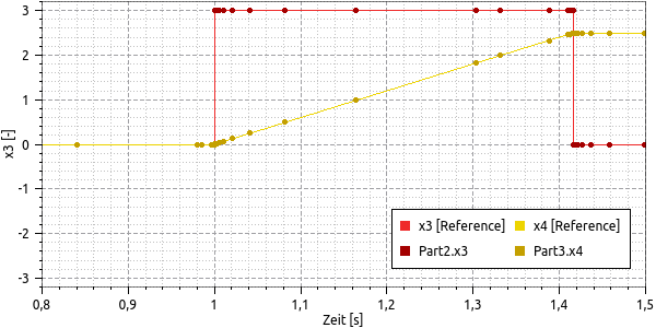
The publication mentioned above illustrates the behavior of the simulation using these parameters.
1.8.2. Error control and time step adjustment
If an error test method (ErrorControlMode) is set, a converged step is followed by a local error check. Currently, this error check is based on the step-doubling technique and as such can only be applied if the slaves support FMI 2.0 setting/getting of state functionality.
Basically, the check is done as follows:
- reset slave state to begin of current communication interval
- take two steps (with full master algorithm per step)
- compute error criteria 1 and 2
- reset states back to state after first master algorithm
|
So, the error test requires two more runs of the master algorithm per communication step. For iterative master algorithms, or the Newton algorithm, the overhead for error tests can be significant. |
The mathematical formulas and calculation details of the error check are documented in publication:
Nicolai, A.: Co-Simulation-Test Case: Predator-Prey (Lotka-Volterra) System (see MasterSim Documentation Webpage).
The error check uses the parameters relTol and absTol to determine an acceptable difference between the full and half-step (or their slopes). Depending on the local error estimate, two options exist:
-
the local error estimate is small enough and the time step will be enlarged,
-
the error check failed; the step size will be removed and the entire communication step will be repeated
|
If you use an error checking algorithm in MasterSim, you should set a fallback time step limit. Otherwise, MasterSim may try to resolve the dynamics of the step change by adjusting the time steps to extremely small values. |
1.9. Master algorithms
A master algorithm is basically the mathematical procedure to advance the coupled simulation by one step forward. Such a co-simulation master algorithm has a characteristic set of rules on how to retrieve values from one FMU, when and how these values are passed on to other FMUs, whether this procedure is repeated and the criteria for convergence of iterations.
MasterSim implements several standard algorithms. A detailed discussion of the different algorithms and how the choice of algorithm and parameters affect results can be found in the following publication:
Nicolai, A.: Co-Simulations-Masteralgorithmen - Analyse und Details der Implementierung am Beispiel des Masterprogramms MASTERSIM, http://nbn-resolving.de/urn:nbn:de:bsz:14-qucosa2-319735 (in german)
1.9.1. Gauss-Jacobi
Basic algorithm:
loop over all slaves:
  retrieve all output values

loop over all slaves:
  set all input values
  tell slave to take a step
Gauss-Jacobi is always done without iteration. As shown in the publication (see above), it really doesn’t make sense to use iteration.
|
Instead of using a communication step of 10 seconds and allow for 2 iterations of Gauss-Jacobi, it is more efficient to disable iteration (setting maxIterations=1) and restrict the communication step size to 5 seconds. The effort for the simulation will be exactly the same, yet the simulation will be more accurate (and more stable) with the 5 seconds communication interval. |
1.9.2. Gauss-Seidel
Basic algorithm:
iteration loop:
  loop over all slaves:
    set input values for slave from global variable list
    tell slave to take a step
    retrieve output from current slave
    update global variable list
  perform convergence check
Cycles
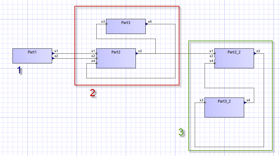
MasterSim includes a feature that reduces the calculation effort when many FMUs are involved and not all are directly coupled. The following figure shows a simulation scenario where calculation can be done in three stages.
| (1) |
This FMU only generates output and can be evaluated first and only once in the Gauss-Seidel algorithm. |
| (2) |
These two FMUs exchange values, they are in a cycle. If the Gauss-Seidel algorithm is executed with iteration enabled, only these two FMUs need to be updated and need to exchange values, since they do not require input from the other FMUs (except for the first one, whose output variables are already known). |
| (3) |
The last two FMUs are also coupled in a cycle, but only to each other. They are iterated in the last stage/cycle. Since the results of the other three FMUs are already computed and known, again only two FMUs need to be in a cycle. |
Restricting the number of FMUs in a cycle not only reduces overall effort, but also takes into account the stiffness of the coupling. In one cycle, FMUs may be loosely coupled, and convergence is achieved in 2 or 3 iterations. In other cycles, FMUs may be coupled in a non-linear relation or react more sensitive to input value changes (= stiff coupling), and 10 or more iterations may be needed. Thus, separating the cycles can significantly reduce computational effort in a Gauss-Seidel method.
Each FMU can be assigned a cycle, which are numbered (beginning with 0) and executed in the order of the cycle number (see simulator definition in section Simulator/Slave Definitions).
1.9.3. Newton
Basic algorithm:
iteration loop:
  in first iteration, compute Newton matrix via difference-quotient approximation

  loop over all slaves:
    set all input values
    tell slave to take a step

  loop over all slaves:
    retrieve all output values

  solve equation system
  compute modifications of variables

  perform convergence check
Cycles are handled just the same as with Gauss-Seidel.
| In the case that only a single FMU is inside a cycle, the Newton master algorithm will just evaluate this FMU once and treat the results as already converged. Of course, in this case no Newton matrix is needed and composed. However, in the (rare) case, that such an FMU connects input values to its own outputs this may lead to problems, since potentially invalid FMU conditions are accepted. |
1.10. Output writing
Outputs are written after each completed step, but only if the time since last output writing is at least as long as defined in parameter hOutputMin.
| If you really want outputs after each internal step, set hOutputMin to 0. |
2. Graphical User Interface
MasterSim has a fairly convenient graphical user interface to define and adjust simulation scenarios. With simulation scenario I mean the definition of which FMUs to import and instantiate as slave (or slaves), how to connect output and input variables, and all properties related to calculation algorithms. Basically, everything that is needed to run a co-simulation.
2.1. Welcome page
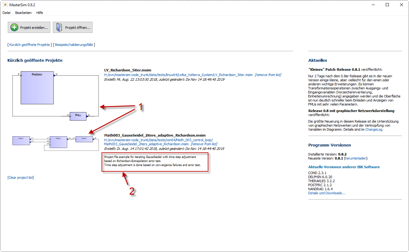
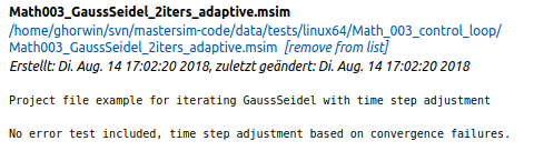
The software starts with a welcome page, which basically shows a list of recently used projects and some webbases news (those are pulled from the file https://bauklimatik-dresden.de/downloads/mastersim/news.html which is updated whenever a new release or feature is available).
| (1) |
Thumbnail with a preview of the simulation scenario |
| (2) |
Short description of the project . This description is taken from the project file header comment lines (see Project file format). |
|
The thumbnails shown on the welcome page are generated/updated when the project is saved. The files are placed inside the user’s home directory:
and the image file is named like the project file with appended |
2.1.1. Examples
When opening an example from the welcome page / example page, you are prompted to save the project first in a custom location (examples are distributed in the installation directory, which is usually read-only).
2.2. Tool bar and useful keyboard shortcuts
As soon as a project is created/opened, one of the project content views is shown, and a tool bar is shown to the left side of the program. The icons of the tool bar have the following functionality (also indicated by a tool tip when hovering with the mouse cursor over the button):
| Programm Information |
Shows program info |
| Create new |
Creates a new project (shortcut Ctrl + N) |
| Open project |
Opens a |
| Save project |
Saves the current project (shortcut Ctrl + S) (also saves the network representation) |
| Open PostProc |
Opens the post processing tool specified in the preferences dialog. While I would recommend to use PostProc 2, you can start here any other postproc software, or even an automated analysis script. Simple set the appropriate command line in the preferences dialog. |
| FMU Analysis |
MasterSim will unzip all referenced FMUs and read their model description files. It also updates the graphical schematics and connection views, if FMU interfaces have changed. Also, the property table is updated. Use this feature if you have updated an FMU in the file system and want to reflect those changes in the MasterSim user interface (alternatively, simply reload the project). |
| Slave definition view |
Switches to the Slaves definition view. Here you define which FMUs are important, and assign parameter values to slaves. Also, you can design a graphic representation of the network. |
| Connection view |
Switches to the Connection view. Here you can manage the connections between slaves and assign special attributes (transformations) between connections. |
| Simulation settings view |
Switches to the Simulation settings view. All simulation parameters and numerical algorithm options are specified here. Also, the actual simulation is started from this view. |
| Undo/Redo |
The next two buttons control the undo/redo functionality of the unse interface. All changes made to the project can be reverted and re-done (shortcuts are Ctrl + Z for undo, and Ctrl + Shift + Z for redo). |
| Language switch |
The next buttons opens a context menu with language selection. You need to restart the application to activate the newly selected language. |
| Quit |
Close the software. If the project has been changed, user is queried to save or discard the changes. |
2.2.1. Useful shortcuts
Here’s a list of useful program-wide shortcuts:
| Windows/Linux | MacOS | Command |
|---|---|---|
Ctrl + N |
CMD + N |
create new project |
Ctrl + O |
CMD + O |
load project |
Ctrl + S |
CMD + S |
save project |
Ctrl + Shift + S |
CMD + Shift + S |
save project with new filename |
Ctrl + Z |
CMD + Z |
undo |
Ctrl + Shift + Z |
CMD + Shift + Z |
redo |
F2 |
F2 |
open project file in text editor |
F9 |
F9 |
start simulation (can be used from any view, no need to switch to simulation settings view first!) |
CMD + . |
Open preferences dialog |
2.3. Slaves definition view
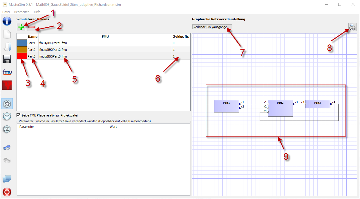
The input of the simulation scenario is split into three views. Setting up a simulation starts with importing slaves. So, the first (and most important) view is the slave definition view.
Items of the view:
| (1) |
Adds a new slave by selecting an FMU file ( |
| (2) |
Removes the currently selected slaves (and all connections made to it) |
| (3) |
Double-click to change color of slave (colour is used to identify slave in connection view) |
| (4) |
ID name of slave. By default MasterSim assigns the basename of the fmu file path. Double-click on the cell to change the same. Mind: slave ID names must be unique within a simulation scenario. |
| (5) |
Path to FMU file, either absolute path or relative to current MasterSim project file, depending in the checkbox "Show FMU paths relative to project file". Also, the project must have been saved, before relative paths can be shown. |
| (6) |
Defines in which cycle the FMU is to be calculated (by default, all slaves are in cycle 0 and thus all are assumed to be coupled). See description of master algorithms. |
| (7) |
Activate graphical connection mode (see discussion below). When this mode is active, you can drag a new connection from an output to inlet socket in the network. |
| (8) |
Print network schematics to printer or pdf file. |
| (9) |
This is the graphical network schematics - purely optional, but helps to understand what you are doing. |
| If you want to rearrange several blocks at the same time, you can select multiple blocks by Ctrl + Click on a block. If you move one of the selected blocks now, the other selected blocks will be moved as well. |
2.3.1. Editing properties of project, selected slave or selected connection
In the lower left part of the view you may edit project comments (if nothing is selected in the network view), slave properties (if a slave is selected, see also Slave properties/parameter values), or connection properties (if a connection is selected).
2.3.2. Adding slaves
New slaves are added by selecting fmu or csv or tsv files. MasterSim automatically uses the basename of the selected file as ID name for the slave. If already such an ID name exists, MasterSim appends a number to the basename. In any case, slave ID names must be unique within the project.
| You can import the same FMU several times. In this case, the slaves will have different ID names, yet reference the same FMU file. Parameters and visual appearance can be set differently for slave of the same FMU. Note, that the FMU must have the capability flag canBeInstantiatedOnlyOncePerProcess set to false in order to be used several times in the same simulation scenario. |
2.3.3. Slave properties/parameter values
Below the table with imported slaves is a list of parameters published by the FMU. The list is specific to the currently selected slave. A simulator slave can be selected in the slave table or by clicking on a block in the network view.
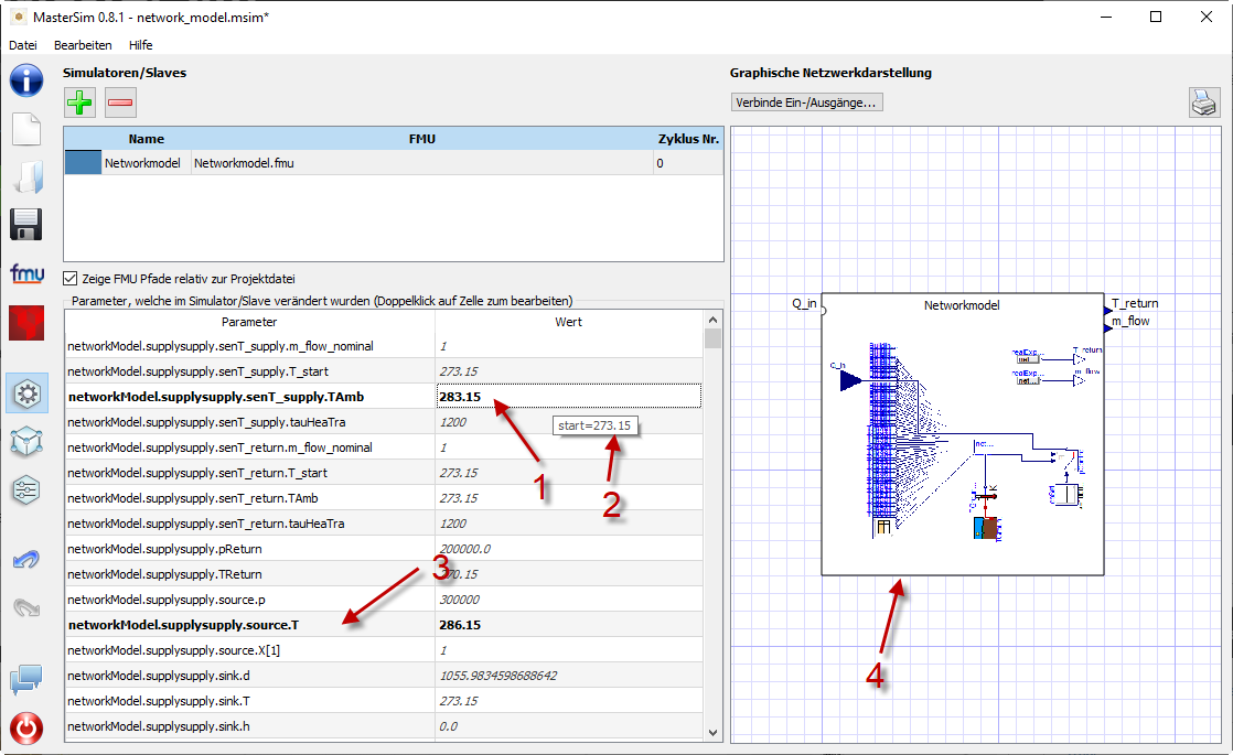
| (1) |
Black and bold fonts indicate, that this parameter has been modified/set to a specific value. Gray italic text shows the default, unmodified value. |
| (2) |
Hovering with the mouse over a parameter value will show a tool tip with the default parameter. This can be used to see the default value in the case that a parameter was modified. |
| (3) |
Parameters written in bold face and black are set by MasterSim (during initialization). |
Parameters can be edited by double-clicking on the value cell and entering a value. Clearing the content of the cell will reset the parameter to its default value.
2.3.4. Network view
The network view (9) shows a simple schematic of all FMU slaves and their connections. This network view is optional and not really needed for the simulation. Still, a visual representation of the simulation scenario is important for communication.
| You can zoom in and out of the network view by using the mouse scroll button. The scene is zoomed in at the position of the mouse cursor. |
The network shows blocks (matching the simulators/slaves) and on each of the blocks one or more sockets. Sockets indicate input/output variables of each simulation slave. Blocks are shown in different colors, indicating the individual block states.
Creating connections in network view
You can create new connections between slave’s outputs and inputs by dragging a connection from an outlet socket (triangle) to a free inlet socket (empty semi-circle). Once the connection has been made, the newly created connection line is shown.
Connections between slaves can be defined more conveniently in the Connection view (which is also more efficient when making many connections, compared to manually dragging the connections with the mouse).
Block states
Because MasterSim only references FMUs, their actual content (i.e. interface properties from modelDescription.xml) is only known when they are imported. The FMU import and analysis step is done automatically, when a project is opened and when a new FMU slave is added.
When importing an FMU the user interface will attempt to unzip the FMU archive and analyse its content. If the modelDescription.xml file could be read correctly, MasterSim will offer to open the block editor. Inside the editor you can define the basic geometry of the block (slave representation) and the layout of the sockets (the positions of inlet and outlet variables). You can ignore this request and leave the FMU visual representation undefined. Basically, an FMU can have three states that are visualized differently in the UI:
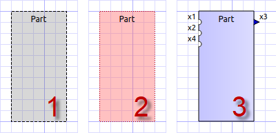
| (1) |
The referenced |
| (2) |
The model description has been parsed successfully for this slave, but the block definition doesn’t match the interface (yet). Typically, when an FMU has been imported the first time, the corresponding block definition does not yet have any sockets defined or layed out, so simply a red box is shown. You can double-click on such a box to open the block editor. |
| (3) |
The block has been defined and the sockets match those indicated by the model description (in name and inlet/outlet type). |
2.3.5. Block editor
The block editor allows you to define the basic, rectangular shape of your FMU and to layout your sockets. The block editor is opened either directly after an FMU has been imported, or when double-clicking on a block in the network view.
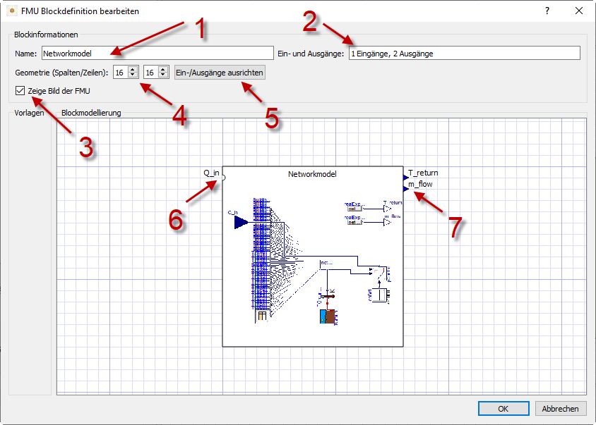
| (1) |
Slave ID name |
| (2) |
Shows number of published input and output variables |
| (3) |
If checked, the FMU archive is searched for the image file |
| (4) |
Here, you can define the width and height of the block in grid lines |
| (5) |
This button will automatically lay out the sockets. Inputs are aligned to the left and top side. Outputs are aligned at the right and bottom side. If there is not enough space for all sockets, the remaining sockets are placed over each other. |
| (6) |
Indicates an inlet socket (input variable) |
| (7) |
Indicates an outlet socket (output variable) |
| In one of the next program versions, it will be possible to store block appearances as templates for future use of similar/same FMUs. For now, you have to configure the block every time you import an FMU. Also, advanced customization and custom socket locations is not yet implemented. |
2.4. Connection view
In this view you can connect slaves by mapping output to input variables.
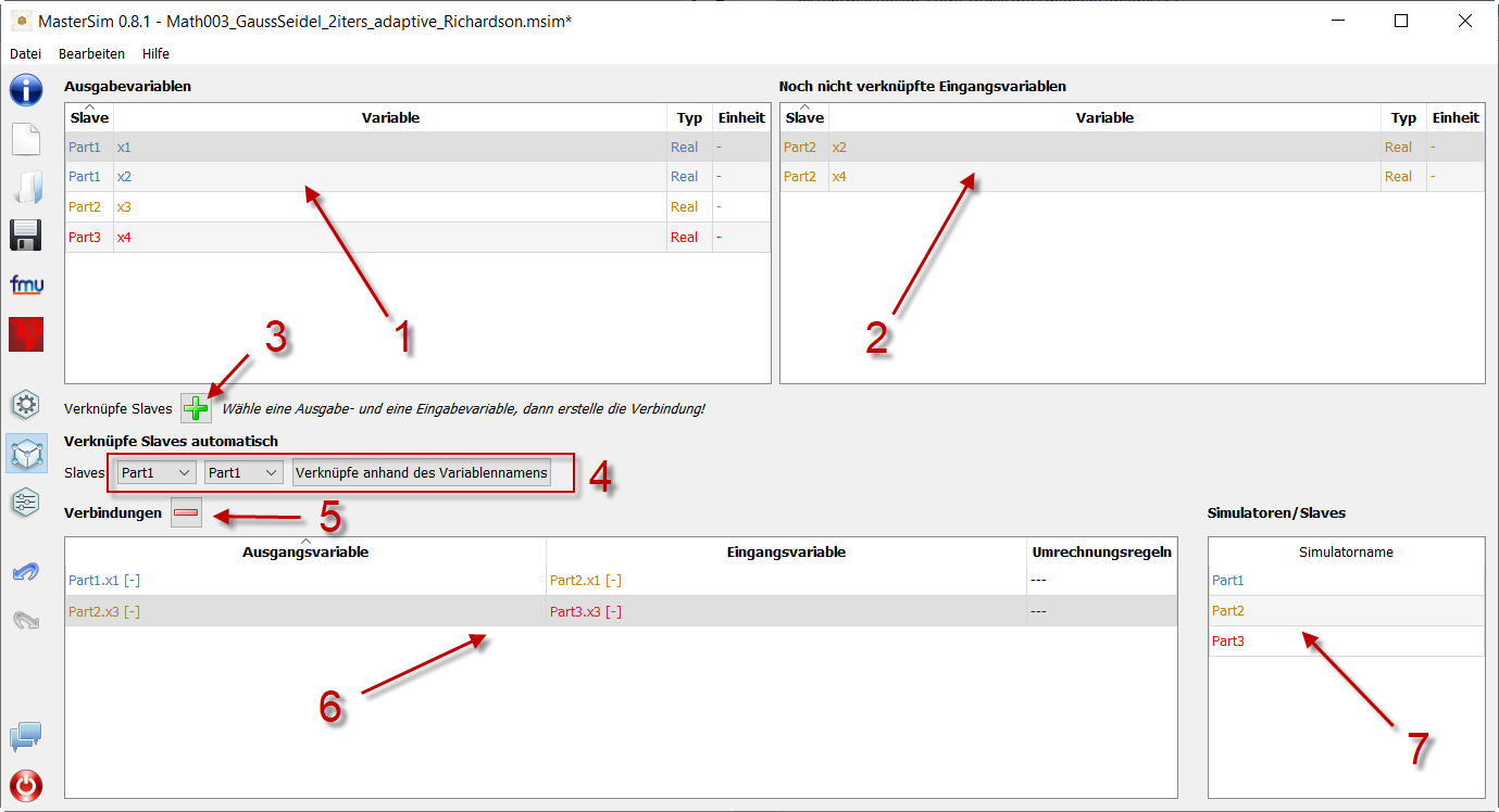
| (1) |
Shows all published output variables of all slaves. |
| (2) |
Shows input variables of all slaves, that have not been connected, yet. |
| (3) |
Select first an output variable and the input variable, that should be connected to the output, then press this button to create the connection. |
| (4) |
Here, you can create multi connections between two slaves based on variable names (see explanation below) |
| (5) |
This removes the currently selected connection in table (6) |
| (6) |
Shows all connections already made. Double-click on last column to assign transformation operations. |
| (7) |
Table with all slaves and their colors (to assist in identifying variables by colour) |
2.4.1. Auto-connection feature
This feature is very helpful if FMUs are coupled, where output and input variables of two slaves have the same name. This is particularly helpful, if you have to connect many input and output variables between two slaves. If you create one FMU such, that variable names match the other side, you can use the following procedure:
-
in the combo boxes select the slaves to be connected
-
press the connection button
A connection is created, when:
-
the variable name matches
-
the variable data type matches
-
one variable has causality input, and the other has causality output
-
slave1 publishes:
-
Room1.Temperature (real, output)
-
Room1.HeatingPower (real, input)
-
Room1.OperativeTemperature (real, output)
-
-
slave2 publishes:
-
Room1.Temperature (real, input)
-
Room1.HeatingPower (real, output)
-
Room2.OperatingTemperature (real, input)
-
Auto-connection creates:
-
slave1.Room1.Temperature → slave2.Room1.Temperature
-
slave1.Room1.HeatingPower → slave2.Room1.HeatingPower
Third connection is not made, since Room1.OperativeTemperature does not match Room2.OperatingTemperature.
2.4.2. Assigning transformation operations to a connection
If you want to do unit conversion or other transformations (sign inversion, scaling) between output variables and input variables, you can double-click on the third column in table (6), to open a dialog for editing transformation factors and offsets. See section Connection graph for a detailed description.
|
You can easily assign conversion operations in the network schematics in the slave view. Simply select the connection to modify and edit the scale factor and offset in the lower left property window. |
2.5. Simulation settings view
All settings that control the actual co-simulation algorithm are defined here. Detailed description of the settings and their usage is given in section Master Algrithms.
| Section Project file reference - Simulator settings describes the corresponding entries in the MasterSim project file. |
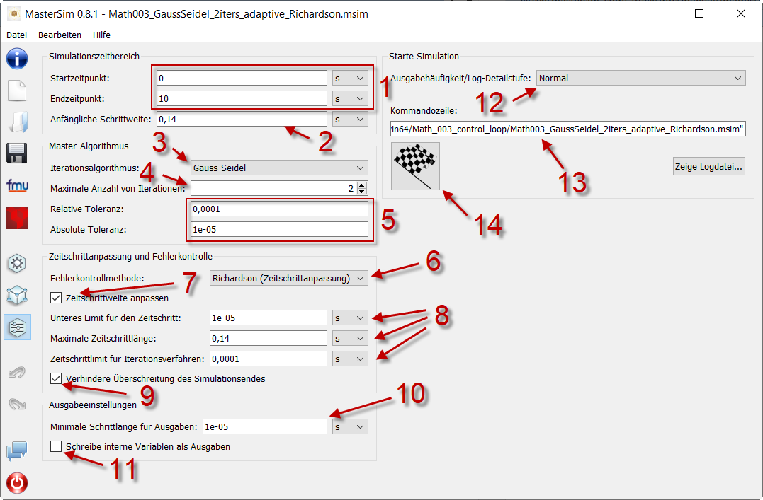
| (1) |
Here you can define the start and end time point of the simulation. |
| (2) |
The initial communication interval size. When time step adjustment (7) is disabled, this communication interval size will be used until the end simulation time has been reached. |
| (3) |
Selection of the master algorithm |
| (4) |
Maximum number of iterations, 1 disables iteration |
| (5) |
The relative and absolute tolerances are used for converence check of iterative algorithms and, if enabled, for local error checking and time step adjustment. |
| (6) |
Here you can select an error control method, see section Error control and time step adjustment. |
| (7) |
If checked, MasterSim will adjust the time step, requires FMUs to support the canHandleVariableCommunicationStepSize capability |
| (8) |
These three parameters control how the time step is adjusted in case of convergence/error test failures. |
| (9) |
If checked, MasterSim will adjust the step size of the last interval such, that it gives exactly the end time point of the simulation as end of the last communication interval, regardless of flag (7) (see discussion in section Time step adjustment). |
| (10) |
Defines the minimum interval that needs to pass before a new output is written. Helps to reduce amount of outputs in case of variable time steps when these time steps can become much smaller than a meaningful output grid. |
| (11) |
If checked, MasterSim also writes the values of internal variables to the output files, otherwise only variables of causality output. Useful mainly for debugging/FMU analysis, or to obtain internal values that are not written to output files by the FMU itself. |
| (12) |
Lets you control the verbosity level of the console solver output (see Command line arguments) |
| (13) |
Command line that is used to run the simulator. Can be copied into a shell script or batch file for automated processing. |
| (14) |
The big fat start button. Ready, Steady, Go! |
When you start the simulation, a console window will appear with progress/warning/error message output of the running simulation. Since some simulations can be very fast, after about 2 seconds the log windows is shown with the current screenlog’s content.
|
Mind, that the simulation may still be running in the background, even if the log window is already shown. If you start the simulation several times, you will spawn multiple simulation processes in parallel. This would just be a waste, since the simulations would write into the same directories and overwrite each other’s files. |
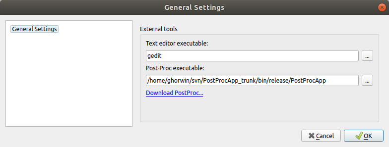
2.6. Preferences Dialog
The preferences dialog, opened from the main menu or via application shortcut, currently provides configuration options for the text editor (used to edit the project file with the short cut F2) and the post processing executable.
| When you edit a project file in the external text editor and save the file, the next time you bring the MasterSim user interface into focus, it will prompt to re-load the modified project. |
3. MasterSimulator - the command line program
The actual simulation is done by the MasterSimulator command line program. It basically performs the following steps:
-
Read the msim project file (the network representation file is ignored, since it only contains visual information).
-
Then, a working directory for the simulation data is created (path can be adjusted, see
--working-dircommand line option below). -
The FMUs are extracted (can be skipped if already extracted, see command line option
--skip-unzipbelow) -
The simulation is run as defined in the project file
3.1. Command line arguments
General Syntax for the MasterSimulator command line tool:
Syntax: MasterSimulator [flags] [options] <project file>

Flags:
  --help            Prints the help page.
  --man-page        Prints the man page (source version) to std output.
  --cmd-line        Prints the command line as it was understood by the command
                    line parser.
  --options-left    Prints all options that are unknown to the command line
                    parser.
  -v, --version     Show version info.
  -x, --close-on-exit  Close console window after finishing simulation.
  -t, --test-init   Run the initialization and stop right afterwards.
  --skip-unzip      Do not unzip FMUs and expect them to be unzipped in
                    extraction directories.

Options:
  --verbosity-level=<0..4>
                    Level of output detail (0-4).
  --working-dir=<working-directory>
                    Working directory for master.
3.1.1. Working/output directory
If no working directory is given, the directory path is generated from the project file path with extension removed. For example:
# path to project file
/simulations/myScenario.msim

# outputs will be written to
/simulations/myScenario/...
In the section Structure and content of the working directory the content of the working directory is explained.
3.1.2. Verbosity of console and log file output
MasterSimulator writes progress information/warning and error messages to the console window, and to the file <working-dir>/logs/screenlog.txt. The amount of text to be written and the detail level is controlled through the --verbosity-level parameter, which determines the amount of debug information generated by the master.
Verbosity level of 0 disables pretty much all output, verbosity level 1 is the default with normal progress message output. Use higher verbosity levels for debugging purposes or to narrow down the source of an error.
|
The log file verbosity is always set to 3 during initialization and reset to the default value of 1 or command line value during simulation (to avoid slowdown of the simulation due to excessive output writing). |
3.1.3. Windows specific options
By default, the console window (on Windows) stays open at the end of the simulation unless the -x command line flag is passed.
3.2. Structure and content of the working directory
By default, the following directory structure is used. Suppose there is a project file simProject.msim describing the simulation scenario using two provided FMUs part1.fmu and part2.fmu which are referenced inside the project as simulation slaves P1 and P2, respectively. Let’s assume these files are located in some subdirectory:
/sim_projects/pro1/simProject.msim
/sim_projects/pro1/fmus/part1.fmu
/sim_projects/pro1/fmus/part2.fmu
When running the master simulator a working directory will be created. By default the file path to this working directory is the project file name without extension.
/sim_projects/pro1/simProject/             - working directory
/sim_projects/pro1/simProject/log/         - log and statistic files
/sim_projects/pro1/simProject/fmus/        - unzipped fmu subdirectories
/sim_projects/pro1/simProject/fmus/part1   - unzipped part1.fmu
/sim_projects/pro1/simProject/fmus/part2   - unzipped part2.fmu
/sim_projects/pro1/simProject/slaves/      - output/working directory for fmu slaves
/sim_projects/pro1/simProject/slaves/P1    - output directory for slave P1
/sim_projects/pro1/simProject/slaves/P2    - output directory for slave P2
/sim_projects/pro1/simProject/results/     - base directory for simulation results
The base directory name, here simProject may be changed by using the --working-directory command line argument.
3.2.1. Directory log
This directory contains three files:
progress.txt-
contains overall simulation progress
screenlog.txt-
contains the output of MasterSim written to the console window with the requested verbosity level (during initialization, always detailed output is written to the logfile, even if nothing is written on the screen due to low verbosity level)
summary.txt-
after the simulation has completed successfully, this file contains a summary of the relevant solver/algorithm statistics.
The format of the progress.txt is fairly simple:
   Simtime [s] 	   Realtime [s]	 Percentage [%]
            600	       0.000205	         0.0019
           1200	        0.00023	         0.0038
           1800	       0.000251	         0.0057
           2400	       0.000271	         0.0076
            ...             ...             ...
The file has three columns, separated by a Tab character. The file is written and updated during the simulation run and can be used by other tools to pick up the overall progress and generate progress diagrams (speed/percentage etc.)
The meaning of the different values in the summary.txt are explained in section.
3.2.2. Directory fmus
Inside this directory, the imported FMUs are extracted, each in a subdirectory with basename of the FMU (part1.fmu → part1).
When a MasterSim project references several FMUs with same base name, which are for example in different subdirectories, then it will adjust the extraction path name. Example:
slave1 : /path/to/fmus/s1.fmu
slave2 : /path/to/fmus/s1.fmu                (1)
slave3 : /path/other/project/fmus/s1.fmu     (2)

# _MasterSim_ generates directories
.../fmus/s1
.../fmus/s1_2 (3)| 1 | second instance of same FMU |
| 2 | different FMU with same basename |
| 3 | suffix 2 and 3 etc. is added by MasterSim |
Basically, each fmu file is only extracted once.
|
Skipping the FMU extraction step
MasterSim provides the command line option See also section Modifying/fixing FMU content. |
3.2.3. Directory slaves
Often, non-trivial simulation slaves write their own output files, instead of pushing all output data via FMI output variables to the master. In cases, where PDEs are solved and many thousands of variables are generated, this may actually not be possible.
Since a slave FMU may be instantiated several times, hard-coding output paths inside the FMU is generally a bad idea (though still current practice). Also, writing outputs into the current working directory is not too smart either, since the working directory would have to be changed by the master between calls to FMUs, and this is best avoided.
Unfortunately, the FMU standard does not provide an option, to officially set such a result directory. MasterSim handles this by setting the slave-specific directory path in a string parameter named ResultsRootDir, if the FMU declares such a parameter. If there is no value set in the project file for this parameter, then MasterSim will set the path generated for the slave in the working directory. The FMU can rely on the path being created by MasterSim and being writable.
Of course, as with any parameter, you can set manually a value for this parameter.
3.3. Return codes of MasterSimulator program
MasterSimulator returns:
| 0 |
upon success |
| 1 |
upon failure (anything from bad or missing FMUs, or errors during calculation, …), |
3.4. Simulation output
3.4.1. Slave output values
MasterSim creates two result files within the results subdirectory.
values.csv-
Number outputs of all output variables of all slaves (whether they are connected or not).
strings.csv-
Values of all output variables of type string of all slaves.
and depending on whether synonymous variables are defined in the ModelDescription (see below), the file synonymous_variables.txt.
String output files are only generated when outputs of this type are generated. CSV files use tab chars as separators. First column is always the time point, the column header indicates the time unit.
Example values.csv file:
Time [s] 	slave1.h [-] 	slave1.v [-]
0	1	0
0.001	0.999995099905	-0.0098100000000001
0.0019999999999999	0.99998038981	-0.019619999999999
0.0030000000000001	0.999955869715	-0.029430000000002
0.0040000000000002	0.99992153962	-0.039240000000001
The file format corresponds to that of the csv-files used as FileReader-slaves, see section CSV FileReader Slaves, with:
-
tabulator separated columns,
-
numbers written in english number format, and
-
a single header line identifying the variables.
The FMI variable names are prefixed with the corresponding slave name. The units are given in brackets and for unitless integer and boolean data types, the unit [-] is used.
Synonymous variables
Some FMUs (i.e. those generated from Modelica models) may have several (internal) variables that share the same value reference. This happens, when the symbolic analysis of the Modelica model has identified those variables as the same. In this case, MasterSim does not write duplicate output variables (would be a waste of harddrive space and simulation time, see ticket #47), but instead create a file synonymous_variables.txt with a table of synonymous variables.
The table is written as plain text file with tab-separated columns:
-
fmu filename (currently, only the file name is written - in case that the same filename with different file paths is being used, this may need to be changed)
-
the name of the variable that appears in the
values.csvfile -
the synonymous variable, that is not written into the output file, since it has the same value anyway
Example for synonymous_variables.txt file:
ControlledTemperature.fmu	heatCapacitor.T	heatCapacitor.port.T
ControlledTemperature.fmu	heatCapacitor.T	heatingResistor.T_heatPort
ControlledTemperature.fmu	heatCapacitor.T	heatingResistor.heatPort.T
ControlledTemperature.fmu	heatCapacitor.T	temperatureSensor.port.T
ControlledTemperature.fmu	heatCapacitor.T	thermalConductor.port_a.T
ControlledTemperature.fmu	heatingResistor.p.v	heatingResistor.v
ControlledTemperature.fmu	heatingResistor.p.v	idealSwitch.n.v
ControlledTemperature.fmu	constantVoltage.i	constantVoltage.n.i
ControlledTemperature.fmu	constantVoltage.i	constantVoltage.p.i
ControlledTemperature.fmu	constantVoltage.i	heatingResistor.i
ControlledTemperature.fmu	constantVoltage.i	heatingResistor.n.i
ControlledTemperature.fmu	constantVoltage.i	heatingResistor.p.i
ControlledTemperature.fmu	constantVoltage.i	idealSwitch.i
ControlledTemperature.fmu	constantVoltage.i	idealSwitch.n.i
ControlledTemperature.fmu	constantVoltage.i	idealSwitch.p.i
ControlledTemperature.fmu	heatingResistor.LossPower	heatingResistor.heatPort.Q_flow
ControlledTemperature.fmu	fixedTemperature.port.Q_flow	thermalConductor.Q_flow
ControlledTemperature.fmu	fixedTemperature.port.Q_flow	thermalConductor.port_a.Q_flow
ControlledTemperature.fmu	fixedTemperature.port.Q_flow	thermalConductor.port_b.Q_flow
ControlledTemperature.fmu	onOffController.reference	ramp.y
ControlledTemperature.fmu	onOffController.u	temperatureSensor.T
ControlledTemperature.fmu	idealSwitch.control	logicalNot.y
ControlledTemperature.fmu	logicalNot.u	onOffController.y
3.4.2. Final statistics/summary
MasterSim contains internal profiling functions that monitor the evaluation times of various parts of the software. Also, execution counts for different critical functions are shown.
The statistics is printed on the console window (for verbosity level > 0) and in the log file screenlog.txt in the following format:
Solver statistics
------------------------------------------------------------------------------
Wall clock time                            =   78.044 ms
------------------------------------------------------------------------------
Output writing                             =   76.767 ms
Master-Algorithm                           =    0.666 ms         324
Convergence failures                       =                      41
Convergence iteration limit exceeded       =                      41
Error test time and failure count          =    0.214 ms          85
------------------------------------------------------------------------------
Part1                               doStep =    0.101 ms        1229
                                  getState =    0.070 ms        1116
                                  setState =    0.020 ms         509
Part2                               doStep =    0.079 ms        1496
                                  getState =    0.039 ms        1116
                                  setState =    0.024 ms         776
Part3                               doStep =    0.071 ms        1496
                                  getState =    0.038 ms        1116
                                  setState =    0.040 ms         776
------------------------------------------------------------------------------
Also, the same statistics information is printed into the summary.txt log file, in a more machine-friendly format (with timings always in seconds):
WallClockTime=0.078044
FrameworkTimeWriteOutputs=0.076767
MasterAlgorithmSteps=324
MasterAlgorithmTime=0.000666
ConvergenceFails=41
ConvergenceIterLimitExceeded=41
ErrorTestFails=85
ErrorTestTime=0.000214
Slave[1]Time=0.000191
Slave[2]Time=0.000142
Slave[3]Time=0.000149
- Wall clock time
-
total simulation time spend after initialization. Time for unzipping and loading of shared libraries is excluded (
WallClockTime). - Output writing
-
time spent in writing output files and computing values related to such outputs (
FrameworkTimeWriteOutputs) - Master-Algorithm
-
Time spent in the actual master algorithm (
MasterAlgorithmTime) and number of calls to the algorithm and overall time steps taken (MasterAlgorithmSteps) - Convergence failures
-
Number of times an iterative master algorithm failed to converge within the allowed number of iterations or diverged. Only applies to iterative master algorithms (
ConvergenceFails) - Convergence iteration limit exceeded
-
Number of times an iterative master algorithm failed to converge within the allowed number of iterations (should be less or equal to convergence failure count). Only applies to iterative master algorithms (
ConvergenceIterLimitExceeded) - Error test time and failure count
-
Number of times the error test failed (
ErrorTestFails) and overall time needed for performing error tests, including the time for resetting FMU states and re-evaluating steps (ErrorTestTime). Only applies to master algorithms with enabled error control (Richardson-variants).
The remaining lines show timings and counters for each slave individually. This lines show the time taken in the function calls to doStep(), getState() and setState() for this slave and the respective call count. The state-related functions are only used by iterative master algorithms, when the FMUs support FMI 2.0 features. Mind, these functions are called both by the master algoritm and by the error test (if enabled).
Output writing and Master-Algorithm are the major two components of the MasterSimulator program, so there times should sum up close to the total wall clock time.
The third column in the screenlog-statistics contains counters. The counter for Master-Algorithm is the number of times the master algorithm takes a step, so that’s the total step count. Re-tries and iterations within the master algorithm are not counted here.
The last section of the statistics lists timings and counters for individual FMU slaves and the most relevant functions.
|
You may use these profiling values to tune your simulation and identify, in case of very slow simulations, which of the FMUs is taking up most of the time. Also, it helps identifying if one of the fast functions (get and set state) are taking way too much time. |
4. Project file format
MasterSim uses a single project file that describes a simulation scenario. This project file has the extension msim and contains all data to perform a simulation.
A second file with same name and extension bm may be present in the same location as the project file. This contains the graphical representation of the simulation scenario. Since the graphical network display is purely optional, the bm file can be omitted/ignored/deleted at will.
|
Future development work
Currently, research is underway within the Modelica Association Project SSP System Structure and Parameterization of Components for Virtual System Design to define a standard for describing simulation scenarios. In due time, when the specs are complete enough, this master simulator may support this file standard, at least for exporting and importing such data. Such a file actually merges description of the FMU connection topology and its (still optional) graphical representation into one file. However, similar to FMUs this file format is actually a zip-compressed folder structure and hence SSP-project files may no longer effectively been used in version control systems. Here, the ASCII format of the current |
The format is a plain-text format (UTF8-encoded) with the following content:
# Created:	Di. Aug. 14 17:02:20 2018
# LastModified:	Di. Aug. 14 17:02:20 2018

# Project file example for iterating GaussSeidel with time step adjustment
#
# No error test included, time step adjustment based on convergence failures.
tStart                   0 s
tEnd                     12 s
hMax                     30 min
hMin                     1e-06 s
hFallBackLimit           0.001 s
hStart                   1e-07 s
hOutputMin               0.12 s
adjustStepSize           no
preventOversteppingOfEndTime yes
absTol                   1e-06
relTol                   0.01
MasterMode               GAUSS_JACOBI
ErrorControlMode         NONE
maxIterations            1
writeInternalVariables   yes

simulator 0 0 Part1 #ff447cb4 "fmus/simx/Part1.fmu"
simulator 1 1 Part2 #ffc38200 "fmus/simx/Part2.fmu"
simulator 2 1 Part3 #ffff0000 "fmus/simx/Part3.fmu"

graph Part1.x2 Part2.x2
graph Part1.x1 Part2.x1
graph Part2.x3 Part3.x3
graph Part3.x4 Part2.x4

parameters Part1.para1  14.3
Each line defines a different property. Tokens in each line are separated by whitespaces (tabs or spaces). Lines beginning with a hash character # are comment and ignored.
All comment lines before the first actual input line are recognized as the header lines. In these lines the keywords Created: and LastModified: are expected to be followed by a more or less meaningful (but not standardized) date/time string to be shown in the user interface. Other header lines are treated as project description, show in the project summary on the welcome page of the graphical user interface (see Figure Project properties shown on the welcome page).
|
Past the header with the description, the order of the entries/lines in the file is arbitrary. |
4.1. Simulator settings
Below is a short description of the different parameters with a format description and what values are needed. For details on where there are used and what influence they have, see section Master Algorithms.
Parameters are given as numbers followed by a unit, except for counters (iteration limit) or tolerances (which are unitless anyway).
Time step related options:
| tStart |
(default=0 s) start time point of simulation |
||
| tEnd |
(default=1 a) end time of simulation, must be > tStart |
||
| hMax |
(default=30 min) maximum time step size |
||
| hMin |
(default=1e-5 s) lower limit of time step in adaptive-time-step mode, if time step is reduced below this limit, master stops |
||
| hFallBackLimit |
(default=1e-3 s) for Gauss-Seidel with time step adjustment: when time step drops below this limit, non-iterating Gauss-Seidel is used (to compensate for discontinous outputs), should be > hMin |
||
| hStart |
(default=10 min) initial time step, will be use as constant step size when not in adaptive-time-step mode.
|
||
| hOutputMin |
(default=10 min) minimum time that need to elapse before next output values are written, if communication step sizes are larger than hOutputMin, outputs may be skipped but the regular output intervals will be kept |
||
| outputTimeUnit |
(default=s) The unit to be used in for the time column (the first column) of output files |
||
| adjustStepSize |
(default=false) enables/disables adaptive-time-step mode, when error control mode is ADAPT_STEP, disabling adjustStepSize is an error |
||
| preventOversteppingOfEndTime |
This flag is needed for certain FMUs, which include a test against surpassing the end simulation time. This is in some cases related to time series parameters, that only last until exactly the simulation end time. Another problem is also, that rounding errors can add to a very small overshooting of the end time point. Nevertheless, well-behaving FMUs should handle overstepping gracefully. Yet, to avoid an FMU error and abort of the simulation, MasterSim can adjust the last communcation interval’s size such, that exactly the end time of the simulation is given to the FMU. If this flag is enabled, the last interval’s step size may be adjusted, even though time step adjustment is generally disabled by flag adjustStepSize. |
MasterMode (default=GAUSS_SEIDEL) is one of:
| GAUSS_JACOBI |
Gauss-Jacobi algorithm (non-iterative) |
| GAUSS_SEIDEL |
Gauss-Seidel algorithm (iterative or non-iterative depending on maxIterations) |
| NEWTON |
Newton algorithm with difference-quotient approximation to Jacobi matrix |
Iteration and convergence parameters:
| maxIterations |
(default=1=disabled) max. number of iterations, if == 1 no iteration is done |
| absTol |
(default=1e-5) absolute tolerance for convergence/error test |
| relTol |
(default=1e-6) relative tolerance for convergence/error test |
ErrorControlMode (default=NONE=disabled) is one of:
| NONE |
no error checking and adjustment |
||
| CHECK |
- only error checking, protocols time and magnitude of exceeded error limit. Also works with FMI 1 (by using the data of the last two steps).
|
||
| ADAPT_STEP |
implicitely enables adaptive-time-step mode and adjusts time step when error limit is exceeded |
4.1.1. Advanced settings
The following settings are mostly needed for use with cross-check procedure.
| preventOversteppingOfEndTime |
(default=true) even for constant-step FMUs, truncate the final step to hit the end time point exactly (needed for some FMUs who have strict end time checking) |
| writeInternalVariables |
(default=false) Also writes variables with local/internal causality (when set to no, only variables with causality output are written) |
Depending on the selected options, certain capabilities must be supported by the FMUs, see section Master Algorithms.
4.2. Simulator/Slave Definitions
Each slave is defined by:
simulator <priority> <cycle> <slave-name> <html-color-code> <path/to/fmu-file>
The cycle indicates whether slave belongs to a cycle with other FMUs. slave-name must be a unique identifier for the slave (see discussion in section Master Algorithms).
| The priority is used to select order of execution within a cycle (for Gauss-Seidel). However, this feature is currently not implemented and slaves within the same cycle are evaluated in the order they are defined. |
The slave/simulator name is a unique identifier of the FMU instance.
|
Slave names must not contain spaces or dots. If a slave name contains a space or a dot, the parser of the project file will state that the simulator definition line is invalid. Also, slave names are used for directory names (target directories for slave-specific output). Hence, they must not contain characters that are not allowed in file system names. |
The html-color-code is a typical html color definition, beginning with a hash character and then either 8 or 6 characters, for example: #ff00ff00 or #00ff00 for green. In the 8 character format, the first hex number is the alpha value (opaqueness - ff = fully opaque, 0 = fully transparent). Currently, there is no use for this value in the user interface, so the 6 character variant is the typical choice.
Last argument in the line is the file path reference to the actual FMU file. The path to FMU file must be enclosed in double-quotes, if the path or filename contains spaces. The path can be absolute or relative to the msim project file. Several slaves can be instantiated from the same FMU file (if the FMU supports this feature). In this case, several simulator lines reference the same FMU file path.
4.2.1. CSV FileReader Slaves
Instead of an FMU, you can also reference a data file (extension tsv or csv). In this case, MasterSim will instantiate FileReader slaves and the data in the file is treated like an FMU that provides only output, but has no input and no parameters.
MasterSim actually supports two flavours of csv files. In both variants, numbers are always written in english number notation. The file parser first attempts to use the tab-separated value flavour by splitting the first two lines at the tab characters. If this yields more than two columns and the same nummber of columns in both lines (the header and first data line), a tab-separated csv/tsv flavour is assumed. Otherwise, the Excel-type quoted-csv flavour is assumed.
Tab-separated values
The format of such an input file follows the same conventions as the file format supported by PostProc2.
The file starts with a single line (the header), identifying variable name and unit in format like:
Time [<time unit>] <tab> <var1 name> [<unit>] <tab> <var2 name> [<unit>]
where <tab> is the tabulator character.
Time [d] <tab> T_lab [C] <tab> T_sample [C] <tab> RH_lab [%]
Example file:
Time [h]     T_lab [C]     T_sample [C]     RH_lab [%]
0            20            20.2             46
0.5          20.1          20.3             43
1.0          22            25               40
3.0          19            15               65
The variable names are the strings in the header line excluding the units (if given). In the example above, the file would provide output variables of with names T_lab, T_sample and TH_lab.
|
A file with this format is automatically obtained if a table with such data is copied & pasted from Libreoffice-Calc/Excel/… into a plain text editor. |
Comma-separated with quotes
In such a file the separation character is the , (comma), and values are quoted using double-quotes. For example:
"time","T_lab [C]","T_sample [C]","RH_lab [%]"
"0","20","20.2","46"
"0.5","20.1","20.3","43"
"1.0","22","25","40"
4.2.2. Time points and time unit
The time points can be spaced at arbitrary intervals. MasterSim currently expects simulations to run in seconds as base time unit. That means, internally, variables are exchanged matching a simulation time in seconds. When an input file defines a different unit for time, MasterSim converts these times into seconds.
The following time units are recognized by MasterSim:
-
ms - milliseconds
-
s - seconds
-
min - minutes
-
h - hours
-
d - days
-
a - years (regular years, 365 regular days, no leap year/day)
|
Default time unit is seconds
In case of missing time unit in the header of the first column, MasterSim currently implies unit seconds (s). |
4.2.3. Interpretation of data provided in FileReader slaves
Variables without given units, i.e. the […] is missing in the column captions, are assigned an unknown/undefined unit -.
|
The variables exported from such a FileReader slave have not yet data types assigned. During the initialization, MasterSim looks at the connections made to FileReader slave variables and assigns data types to the variables based on the connected input variable. |
During simulation, when the FileReader slave is asked to provide a value for a variable, the following rules apply.
Boolean, Integer and Enumeration values
For Boolean, Integer and Enumeration values no interpolation is done. Values are returned constant until the value is defined to change. Example:
Time [s]   Value [-]
 1         4
 3         4 (1)
 3         7 (2)
 6         4
| 1 | Value at end of interval ending at time 3 |
| 2 | Value at begin of interval beginning at time 3, this value shall be used from t>=3. |
Evaluation of these values yields:
v(1) = 4
v(2) = 4
v(2.99999) = 4
v(3) = 7
v(4) = 7
v(5.99999) = 7
v(6) = 4
Thus, the line 3 4 could have been omitted from the file.
Real values
Real values are linearly interpolated. For the data example above, real values would be evaluated as follows:
 v(1) = 4
 v(2) = 4
 v(2.99999) = 6.99999 (1)
 v(3) = 7
 v(4) = 6 (2)
 v(5.99999) = 4.00001
 v(6) = 4
| 1 | When duplicate time points are found, the second overwrites the first, so that the line 3 4 is ignored. Hence, evaluation of values in the interval 2…3 is also done with linear interpolation. |
| 2 | The linear interpolation between values v(3)=7 and v(6)=4 at t=4 yields 6. |
If you want to emulate step functions with Real values, just use a very short change interval, for example v(1) = 4; v(2.9999) = 4; v(3) = 7. MasterSim will still see the linear slope between t=2.9999 and 3, but that may be insignificant to the results.
|
Naturally, for string parameters linear interpolation is not possible, thus they are handled similarly as integer values.
|
If you use an adaptive step algorithm in MasterSim, you should set the maximum time step/communication interval length to a value that is less than your smallest time interval in your FileReader slave input file. Otherwise, MasterSim may adjust time steps to a larger value and jump over an interval/value, hereby missing information and likely generating wrong results. For example: if you work with hourly climatic data, choose 30 minutes as maximum communication interval length. |
4.3. Connection graph
The connection graph defines data exchange between slaves. Each graph definition line defines the data transfer from one output variable to one input variable.
Definition syntax:
graph <outputvar> <inputvar> [<offset> <scale factor>]
Output and input variables are composed of slave name and variable name:
graph <slave-name>.<variable-name> <slave-name>.<variable-name> [<offset> <scale factor>]
The offset and scale factor define a transformation operation between the output variable and the value given to the input variable. If such a transformation is assigned to a connection, always both values must be present.
The following transformation equation is applied:
input = offset + scale * output
If, for example, an FMU slave Sensor delivers a temperature in Kelvin, and another FMU slave Heater takes a temperature in degree Celsius, you could define the connection as follows:
graph Sensor.temperature Heater.temperature -273.15 1
which will result in
input (in C) = -273.15 + 1 * output (in K)
Similarly, you can invert the sign of a connection, when you, for example, connect heat or mass flows across pipes. Suppose heat flow is defined positively into a surface and you connect SurfaceA.HeatFlow and SurfaceB.HeatFlow, the connection with sign inversion is defined as:
graph SurfaceA.HeatFlow SurfaceB.HeatFlow 0 -1
4.3.1. FMU Parameters
You can set parameters of FMUs (or more specifically of the individual FMU slaves/instances) by using the parameter keyword.
Definition syntax:
parameter <slave-name>.<variable-name> <value>
For boolean parameters you have to specify true (case-sensitive!) for true, or any other value (for example false) for false.
For integer values you specify simply the value as number.
Values for Real parameters are expected in the unit defined for the respective parameter in the modelDescription.xml file. Unit conversion is not supported here.
For string parameters, everything after the variable name is taken as string (until end of line). Example:
parameter building_model.projectFile C:\\My projects\\p2\\This tall building.project
Whitespaces can be included, but backspaces need to be encoded as \\. Line breaks have to be encoded with \n, as in the following example:
parameter building_model.configPara First line\n Some more lines with indentation\nlast line.
Will set the string:
First line
    Some more lines with indentation
last line
|
Because of the rather simple string encoding, you cannot define a string that starts with a whitespace character. |
4.4. BlockMod - Network Representation File Format
The bm file is a simple xml file and describes the graphical layout and visualization of the modeled simulation scenario.
A simple network like
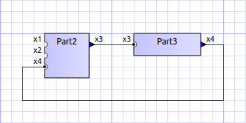
is defined in the following BlockMod network representation file:
<?xml version="1.0" encoding="UTF-8"?>
<BlockMod>
	<!--Blocks-->
	<Blocks>
		<Block name="Part2">
			<Position>224, -160</Position>
			<Size>64, 64</Size>
			<!--Sockets-->
			<Sockets>
				<Socket name="x1">
					<Position>0, 16</Position>
					<Orientation>Horizontal</Orientation>
					<Inlet>true</Inlet>
				</Socket>
				<Socket name="x2">
					<Position>0, 32</Position>
					<Orientation>Horizontal</Orientation>
					<Inlet>true</Inlet>
				</Socket>
				<Socket name="x4">
					<Position>0, 48</Position>
					<Orientation>Horizontal</Orientation>
					<Inlet>true</Inlet>
				</Socket>
				<Socket name="x3">
					<Position>64, 16</Position>
					<Orientation>Horizontal</Orientation>
					<Inlet>false</Inlet>
				</Socket>
			</Sockets>
		</Block>
		<Block name="Part3">
			<Position>352, -160</Position>
			<Size>96, 32</Size>
			<!--Sockets-->
			<Sockets>
				<Socket name="x3">
					<Position>0, 16</Position>
					<Orientation>Horizontal</Orientation>
					<Inlet>true</Inlet>
				</Socket>
				<Socket name="x4">
					<Position>96, 16</Position>
					<Orientation>Horizontal</Orientation>
					<Inlet>false</Inlet>
				</Socket>
			</Sockets>
		</Block>
	</Blocks>
	<!--Connectors-->
	<Connectors>
		<Connector name="new connector">
			<Source>Part2.x3</Source>
			<Target>Part3.x3</Target>
			<!--Connector segments (between start and end lines)-->
			<Segments>
				<Segment>
					<Orientation>Horizontal</Orientation>
					<Offset>0</Offset>
				</Segment>
			</Segments>
		</Connector>
		<Connector name="auto-named">
			<Source>Part3.x4</Source>
			<Target>Part2.x4</Target>
			<!--Connector segments (between start and end lines)-->
			<Segments>
				<Segment>
					<Orientation>Vertical</Orientation>
					<Offset>80</Offset>
				</Segment>
				<Segment>
					<Orientation>Horizontal</Orientation>
					<Offset>-288</Offset>
				</Segment>
				<Segment>
					<Orientation>Vertical</Orientation>
					<Offset>-48</Offset>
				</Segment>
			</Segments>
		</Connector>
	</Connectors>
</BlockMod>
The format is pretty self-explanatory. The first and last segment are defined automatically depending on the socket position on the block and are hence not stored in the network representation file.
|
BlockMod is an open source library for modeling such networks. The wiki page of the project contains more in-depth information on the data format and functionality. |
5. Test Suite Concept
The MasterSim repository includes a subdirectory data/tests with a regression test suite. These tests are used to check whether all algorithms work as expected and whether changes in the code base accidentally break something.
MasterSim is also run through the FMI cross-checking tests. The files and scripts related to those tests are in the subdirectory cross-check.
5.1. Regression tests
5.1.1. Directory structure
/data/tests                     - root directory for tests
/data/tests/<platform>/<test>   - base directory for a test suite
platform is (currently) one of: linux64, win32,win64 and darwin64
Each test suite has a set of subdirectories:
fmus                 - holds fmu archives needed for the test
description          - (mathematical) description of the test problem
Within a test suite different similar test cases with modified parameters or adjusted solver settings can be stored. Test cases are grouped in test suites mostly when they use the same FMUs or other input files.
For each test case a MasterSim project file exists with the extension msim. The script that runs the test cases processes all msim files found in the subdirectory structure below the current platform.
For a test case to pass the check, a set of reference results must be present, stored in a subdirectory with name
<project_file_without_extension>.<compiler>_<platform>
For example:
FeedthroughTest.gcc_linux
FeedthroughTest.vc14_win64
These directories are basically renamed working directories after a simulation run, where everything except summary.txt and values.csv has been removed.
5.1.2. Running the tests
The tests are run automatically after building with the build scripts. Otherwise run the appropriate script:
-
build/cmake/run_tests_win32.bat -
build/cmake/run_tests_win64.bat -
build/cmake/run_tests.sh
5.1.3. Updating reference results
From within a test directory, call the script update_reference_results.py with the directory suffix as argument.
For example, from within:
data/tests/linux64/Math_003_control_loop
call:
> ../../../../scripts/TestSuite/update_reference_results.py gcc_linuxwhich will update all reference results in this directory. If you want to process/update the reference results of several test suites, execute the following script from one directory up, for example from data/tests/linux64:
> ../../../scripts/TestSuite/update_reference_results_in_subdirs.py gcc_linux5.2. Cross-Checking Rules and FMI Standard.org Listing
See documentation in subdirectory cross-check.
5.3. Ways to generate test FMUs
5.3.1. Custom C++ FMUs
A convenient way to get simple, very specific test FMUs is the use of the FMI Code Generator tool. Its a python tool with graphical interface where FMU variables and properties can be defined. With that information, the code generator creates a source code directory with template code and related build scripts - such that it is very easy to handcraft own FMUs. See documentation/tutorial on the github page.
5.3.2. FMUs exported from SimulationX
Requires a suitable license. Exporting FMUs from SimX is very easy, but limited to the Windows platform.
5.3.3. FMUs exported from OpenModelica
OpenModelica can export FMUs as well. Here are the steps to generate such an FMU.
Create Modelica Model
Create a modelica model.
|
Annotate variables to be used as output quantities with keyword |
For example:
model BouncingBall "The 'classic' bouncing ball model"
  type Height=Real(unit="m");
  type Velocity=Real(unit="m/s");
  parameter Real e=0.8 "Coefficient of restitution";
  parameter Height h0=1.0 "Initial height";
  output Height h "Height";
  output Velocity v(start=0.0, fixed=true) "Velocity";
  output Integer bounceCounter(start=0);
  output Boolean falling;
initial equation
  h = h0;
equation
  v = der(h);
  der(v) = -9.81;
  if v < 0 then
    falling = true;
  else
    falling = false;
  end if;
  when h<0 then
    reinit(v, -e*pre(v));
    bounceCounter = pre(bounceCounter) + 1;
  end when;
annotation(
    experiment(StartTime = 0, StopTime = 5, Tolerance = 1e-6, Interval = 0.01));
end BouncingBall;
Variant 1: Generate FMU manually
First open OMShell, then type the following commands to load the model and generate a co-simulation FMU:
>> loadFile("/path/to/modelica/models/BouncingBall/BouncingBall.mo")
>> translateModelFMU(BouncingBall, fmuType="cs")
"/tmp/OpenModelica/BouncingBall.fmu"
The output indicates that the FMU file /tmp/OpenModelica/BouncingBall.fmu has been successfully created.
For Version 2.0 of FMI standard use:
>> translateModelFMU(BouncingBall, fmuType="cs", version="2.0")Variant 2: Script-based automatic FMU generation
Create a script file (createFMU.mos) with the following content:
loadModel(Modelica, {"3.2.1"}); getErrorString();
loadModel(Modelica_DeviceDrivers); getErrorString();

setLanguageStandard("3.3"); getErrorString();

cd("./fmus");
loadFile("../reference_Modelica/BouncingBall.mo"); getErrorString();

setDebugFlags("backenddaeinfo");getErrorString();
translateModelFMU(BouncingBall, fmuType="cs"); getErrorString();
Run the script via:
> omc createFMU.mos6. Features assisting in FMU development and debugging
This section describes some of the features of MasterSim, that are particularly useful for developers of own FMUs or to identify calculation problems with third-party FMUs.
6.1. Modifying/fixing FMU content
If an FMU has an invalid modelDescription.xml file, the process of unpacking the FMU, fixing the file, packing the FMU again and re-trying the simulation with a co-simulation master may be time consuming. With MasterSim you run the simulation once and get the FMU extracted in the respective fmus subdir. There, you can inspect all files and fix errors, or add missing files.
Next time you run MasterSimulator, pass the command line option --skip-unzip and MasterSim will skip over the unzip step and directly access the files in the extraction directory.
7. Developer information
|
The information provided in this chapter will eventually be moved into the MasterSim Developers Guide. |
7.1. Building the Library and Executables
7.1.1. Building on the command line
Linux/MacOS
cd build/cmake
./build.sh [release] [<number of CPUs>]
See build.sh for more command options. By default, binaries are build in release with debug symbols mode.
In case of missing dependencies (zlib is required) you may want to install the corresponding development packages.
Windows
Convenience scripts are included for building with Visual Studio 2015 and Qt5 (for the user interface of MasterSim). Other compilers such as MinGw work as well, but file paths need to be configured manually.
The files are located in the build/cmake directory:
build\cmake\build_VC.bat (1)
build\cmake\build_VC_x64.bat (2)
| 1 | for x86 builds |
| 2 | for x64 builds |
For the scripts to work, Qt must be installed in the following location:
C:\Qt\5.15.2\msvc2019 (1)
C:\Qt\5.15.2\msvc2019_64 (2)
| 1 | for x86 builds |
| 2 | for x64 builds |
and jom.exe is expected at:
c:\Qt\Tools\QtCreator\bin\jom.exe
Also, cmake must be in the path.
If Qt or JOM is installed elsewhere, the environment variables JOM_PATH and CMAKE_PREFIX_PATH can be set alternatively (see build-batch files).
With this setup, you can now build either in 32-bit or 64-bit mode:
cd build\cmake
build_VC.bat
or
cd build\cmake
build_x64.bat
For different Visual Studio versions or MinGW copy batch file and edit path constants. You may also want to edit these batch files if you have different installation paths.
7.1.2. External Libraries
The MasterSim library and the simulator projects depend on the following external/third-party libraries (except for Qt, all are included in the source code repository, so it is not necessary to install these libraries separately):
MasterSimulator and MasterSimulatorUI
-
IBK library (from IBK, TU Dresden, Germany)
-
IBKMK library (from IBK, TU Dresden, Germany)
-
TiCPP library (adapted version provided by IBK, TU Dresden, Germany)
-
minizip and zlib for unzipping FMUs
only MasterSimulatorUI
-
BlockMod library (from IBK, TU Dresden, Germany, hosted on github)
The release-versions of the libraries (with the exception of Qt) are located in the sub-directory third-party.
The libraries in the third-party subdir are way outdated. Please only use the source code in the externals subdirectory of the repository.
|
7.2. Development environments and project/session files
7.2.1. Qt Creator
Development with Qt Creator is encouraged and project files are provided. Individual project files are in subdirectories
<library/app>/projects/Qt/<library/app>.pro
Executables are placed in
bin/debug        - output path for development with Qt Creator
bin/release      - default output path for cmake-builds
7.2.2. Visual Studio
CMake-generated VC project files
The simplest variant that should always work is to use CMake-generated VC project files and solution.
Basic steps: Open a console window, setup VC build environment and all required paths, then use cmake with the Visual Studio makefile generator.
You can re-use the build.bat or build_x64.bat files for that purpose. Open a command line window and change into the directory build/cmake.
-
start either
build.batorbuild_x64.batand press Ctrl+C once building starts. -
leave subdirectory and create a new subdirectory vc:
> mkdir vc > cd vc -
open cmake gui, given the parent directory as source dir and select a Visual Studio build generator
> cmake-gui ..Afterwards you can open the generated .sln file and start debugging (development is not really recommended in Visual Studio).
7.3. Helpful stuff related to development on Linux
Here are some notes collected when I encountered some unexpected difficulties while creating this master simulator:
7.3.1. Checking symbols in shared libraries
objdump -t <shared_library>
nm [-CD] <shared library>
To get all fmi2 functions
objdump -t <shared_library> | grep fmi27.4. Debugging MasterSim and FMUs
7.4.1. Background on shared library handling on Linux
MasterSimulator can be built in Qt Creator in debug mode. By default the qmake projects will create shared libraries for all dependent libraries like IBK, BlockMod, TiCPP etc.
Slaves can also be built to link against their dependency as shared libraries. This happens, for example, when typical IBK-based projects are also built in debug mode.
Now, since MasterSim and FMU slaves are developed seperately, it is likely that the version of common libraries like IBK, BlockMod, IBKMK etc. differ. This then becomes a problem!
Dynamic linking against shared libraries and LD_LIBRARY_PATH
When launching MasterSimulator, it will search for dynamic libraries like libIBK.so using the environment variable LD_LIBRARY_PATH. Also, when the dynamic library of the slave is loaded, again its shared libraries need to be located. Their paths should also be present in LD_LIBRARY_PATH. However, if the path now includes two locations, each containing a different version of the libIBK.so, the first one found is linked against both MasterSimulator and the slave library. Naturally, this will likely cause undesired behavior and usually result in segfaults.
The same problem may occur even if MasterSimulator is linked statically against its libraries, yet two different FMU slaves are linked dynamically against different versions of the same library (e.g. DELPHIN against IBK 4.9.x and NANDRAD against IBK 5.0.x). Unless the commonly used library uses semantic versioning and stable APIs (for example, library versions with same major and minor version always have identical memory layouts and compilation settings, and thus can be freely exchanged), one has to ensure that only one shared library is in use.
|
Rule of thumb: Avoid dynamic linking completely or use dynamic linking only for one library or the master. |
Basically, one needs to ensure that only one set of shared libraries is being used. There are different options, depending on which part of the software you’d like to develop/debug.
7.4.2. Developing/Debugging MasterSim
When developing MasterSim it is best to compile all FMUs to link statically against their dependencies:
-
MasterSim can be developed on Qt Creator in Debug mode and its dependent libraries as shared libs;
LD_LIBRARY_PATHmust hold the location of these libraries -
FMUs are created with CMake either in release, reldeb or debug mode, but statically linked in any case
7.4.3. Developing/Debugging FMUs
-
MasterSim should be compiled with CMake either in release, reldeb or debug mode, and statically linked against its libraries
-
other FMUs should be linked statically
-
the FMU to be developed can be opened in Qt Creator and linked dynamically against its dependent libraries;
LD_LIBRARY_PATHmust hold the location of these libraries
7.4.4. FMU Debugging Step-by-Step Guide
Assuming you develop the shared FMU library with Qt Creator, you can follow this procedure:
-
build your FMU either in debug mode or release-with-debug-symbols, you can use also an external build tool chain, for example cmake; you can also use an out-of-date version of the FMU library as it will be replaced later anyway
-
compose your FMU and zip it into the fmu archive (you need to do this only once)
-
create your msim test project
-
run MasterSimulator once with the project; it will create the basic directory structure and extract the FMU library into the
project/fmus/xxx/binaries/linux64directory -
now create a symlink to the shared library built by Qt Creator that overwrites the .so file there:
ln -s /path/to/FMU/bin/debug_x64/libFMUSlaveName.so.1.0.0 FMUSlaveName.sowhere
FMUSlaveName.sois the name of the shared lib insidebinaries/linux64 -
in Qt Creator, configure the debugging session by specifying MasterSimulator as executable, setting the commandline to contain
/path/to/project.msim --skip-unzipand set the LD_LIBRARY_PATH environment variable to point to the directory containing any shared libs the FMU links against. -
Start debugging/FMU development…
7.5. Inside MasterSim
7.5.1. Data Types
In simulations with mixed FMUs (v1 and v2) data types should match. Also, the default type-headers are the same for both versions.
Intendet platform for this master is Desktop systems (32bit/64bit), therefore all data types seen by the master algorithms are mapped to:
-
fmi2Boolean(boolin scalar interface functions) -
int -
double -
std::string
7.5.2. Connection Graph and Variable Mapping
Variables can be uniquely identified by
<slave-name>.<variable-name>
and a graph may be defined by:
A.x1         B.u1
A.d1         C.du1
B.x1         C.u1
B.x2         A.u2
C.x1         A.u1
First colum are output variables, second column are connected input variables. x are of type real, d of type integer.
Each slave holds for each data type a vector of output values (bool, int, real/double, string). The master also holds for each data type a vector of connection variables.
A mapping of variables from local slave storage to global vector and from global vector to input is done with a mapping table for each data type individually:
Output mapping - Type Real
| Slave | VariableName | global index | local index |
|---|---|---|---|
A |
x1 |
0 |
0 |
B |
x1 |
1 |
0 |
B |
x2 |
2 |
1 |
C |
x1 |
3 |
0 |
The transfer from local to global data storage is then a simple algorithm:
loop connectedVariableIndexes:
    copy(localArray[localIndex], globalArray[globalIndex])
In case of slave B the array connectedVariableIndexes will be [0, 1].
Input mapping - Type Real
For input variables a similar mapping exists. Each slave does not have an input variable cache, instead variables are set individually (see also Newton algorithm and Jacobian generation via DQ algorithm).
| Slave | VariableName | global index | local value reference |
|---|---|---|---|
B |
u1 |
0 |
55 |
C |
u1 |
1 |
348432 |
A |
u2 |
2 |
122 |
A |
u1 |
3 |
321 |
Input and output mappings are combined into a single table RealVariableMappings.
Note: An output of a slave may be directly connected to any of its own input variables, for example:
fmu1.var2 fmu1.var15