| Validation of Calculation Algorithm applied to 2D-Thermal-Bridge Problems |
The EN 10211:2007 standard provides a procedure for validating thermal-bridge calculation software.
The procedure is listend in the appendix A and requires two cases for 2D simulation programs. DELPHIN, as two-dimensional transient
hygro-thermal simulation program can be used to calculate these cases, as shown below.
When using DELPHIN for steady-state calculations one applies constant boundary conditions and runs the simulation until the transients
resulting from the initial condition disappear. Therefore, the selection of the initial condition has an impact on how long the simulation
should be run. | |
We recommend starting with a short simulation time of a few hours to 2 days, with hourly output steps.
If the monitored variables are still changing, we suggest increasing the simulation time by a factor of 2 or 3 (depending on the magnitude of the variations)
and using the continue/restart feature in DELPHIN. Normally, even complex constructions should arrive at steady-state within a few days of simulation time.
In the simulations done for the EN 10211:2007 validation we had to use sometimes simulation times of up to 40 days
(which also says something about the likelihood that a steady-state result may actually occur in real life :-).
|
| Validation Case 1 |
This validation case requires the calculation of a flat plate, exploiting the symmetry in the calculation. The outputs should be obtained at defined grid points.
In DELPHIN we used a modelling-trick to simplify the grid generation. We defined two materials with the same properties, yet different names. We then created a checkerboard
grid with alternating materials. Now we could use the built-in grid generator, specify minimum element width and stretch factor and generate the grids used for the study.
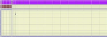
The picture at the side shows one generated grid (click to enlarge).
| | 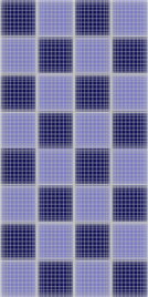 This is the grid generated with 1 mm elements at the boundaries and output nodes, a stretch factor of 1.476, and 15488 elements (control volumes) in total.
|
|
Validation Results and Project
The final project that we used for the validation can be downloaded below. It was tested on DELPHIN versions 5.6.4 and 5.6.5. The next DELPHIN will include
the validation cases as example projects.
EN_ISO_10211_2007_Case1.dpj
(right-click on the link to save the file)
The results obtained are shown in the table along with the original values and the differences. All differences are below the threshold of 0.1 Kelvin.
The first table lists the results obtained with the DELPHIN simulation project. The values in parenthesis are the reference values to match.
| |
9.659 (9.7)   13.385 (13.4)   14.736 (14.7)   15.093 (15.1)
5.249 (5.3)    8.643  (8.6)   10.320 (10.3)   10.815 (10.8)
3.186 (3.2)    5.610  (5.6)    7.017  (7.0)    7.468  (7.5)
2.012 (2.0)    3.641  (3.6)    4.660  (4.7)    5.002  (5.0)
1.261 (1.3)    2.308  (2.3)    2.987  (3.0)    3.219  (3.2)
0.739 (0.7)    1.359  (1.4)    1.767  (1.8)    1.908  (1.9)
0.341 (0.3)    0.629  (0.6)    0.819  (0.8)    0.886  (0.9)
The table below lists the (absolute) deviations of the calculated from the given values.
0.04	0.02	0.04	0.01
0.05	0.04	0.02	0.01
0.01	0.01	0.02	0.03
0.01	0.04	0.04	0.00
0.04	0.01	0.01	0.02
0.04	0.04	0.03	0.01
0.04	0.03	0.02	0.01
|
|
Grid Sensitivity Study
Grid Sensitivity Studies are done to estimate the numerical errors introduced by form and density of the
calculation mesh. This technique allows evaluation of the various parameters that influence the density of
the grid most strongly. In our two cases we investigate the effect of the computational grid on the
calculated temperatures. We modify two parameters, the stretch factor and the minimum element size near
the boundary or material interfaces. Both parameters also change the total number of grid elements.
| |
One of the investigated parameters is the stretch factor. It defines the size ratio of two adjacent elements.
The other defines the minimum width/height of an element at the boundary or material interfaces. By specifying
both parameters, the maximum element size is automatically calculated unless an upper limit is given.
In the first two diagrams both parameters are modified individually. In the third case the mesh density is
increased by modifying both parameters simultaneously.
The horizontal axis shows the number of elements, the minimum element thickness or the stretch factor. The vertical axis
shows the differences in temperature between calculated values and reference temperatures from the standard.
From the 28 points the six most significant or interesting points were selected and shown in the diagram.
|
Figure 1: Modified Stretch Factors
The stretch factor varies between 1.15 and 1.51. The minimum element width was fixed at 1 mm.
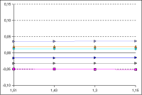
(click to enlarge diagram)
The straight lines indicate that the stretch factor does not have much influence here.
| |
Figure 2: Modified Minimum Element Width
The parameter for the minimum width/height of grid elements at the boundary was varied between 1 mm and 10 mm. The stretch
factor was kept constant at 1.51.
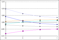
(click to enlarge diagram)
It appears that the element size near the boundary and material interfaces has a major impact on the results. Especially
for large boundary elements the calculated temperatures deviate strongly from the reference/accurate temperatures. For smaller
elements the grid becomes more dense and the calculation errors become smaller.
Beyond a minimum element width of 1 mm a further refinement does not bring much improvement. One can expect that in this case
with 1 mm the calculation accuracy is sufficient.
|
|
Figure 3: General Grid Refinement
The stretch factor is here changed from 1.51 in the coarsest grid to 1.21 for the most dense grid. At the same time the minimum
element size is changed from 10 mm to 1 mm.
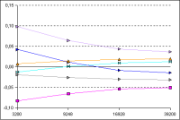
(click to enlarge diagram)
| |
The following table shows the considered cases, and the corresponding total number of elements in the grid.
Case   Elements   min   stretch
  I      3200      10     1,51
 II      9248       5     1,3
III     16928       2     1,3
 IV     39200       1     1,21
The results are nearly identical to the figure for modified minimum element width. It seems that it is more important,
to work with small boundary elements rather than using a overall fine mesh with small stretch factors. The latter leads
to more elements and consequently to longer calculation times, yet hardly more accuracy.
In transient simulations, especially when considering moisture transport, strong gradients can also appear inside the construction.
An example would be a simulation of an adsorption experiment. Here, the stretch factor gains importance again!
|
| Validation Case 2 |
This validation case requires the calculation of 2D detail, composed of concrete, wood, thermal insulation and an aluminum sheet.
The construction was modeled as shown on the picture to the right. Usually, thin metal sheets require a very fine mesh at and near the sheet layers.
Also, small elements near the surface are required to capture the heat fluxes.
Also, the large thermal conductivity differences between materials
will result in slower calculation times and quite long simulations are needed to reach steady-state. Still, even with a very detailed grid the
calculation is done within 3 minutes on a normal PC.
| |
The screenshot below shows the simulation model in DELPHIN without discretization applied (click to enlarge and scroll up).

The next screenshot shows a fairly rough discretization for case 2 with only 6460 elements (click to enlarge and scroll up).
|
|
Validation Results and Project
The final project that we used for the validation can be downloaded below. It was tested on DELPHIN versions 5.6.4 and 5.6.5. The next DELPHIN will include
the validation cases as example projects.
EN_ISO_10211_2007_Case2.dpj
(right-click on the link to save the file)
The results are shown in the table along with the original values and the differences. All differences are below the threshold of 0.1 Kelvin.
| |
The values are given for the different test points. The first value is the one calculation by DELPHIN, the value in parenthesis is
the reference value and the last value is the absolute difference.
A:  7.125 (7.1)    0.025
B:  0.763 (0.8)    0.037
C:  7.967 (7.9)    0.067
D:  6.331 (6.3)    0.031
E:  0.829 (0.8)    0.029
F: 16.384 (16.4)   0.016
G: 16.249 (16.3)   0.051
H: 16.747 (16.8)   0.053
I: 18.328 (18.3)   0.028

Total heat flux:                  9.534 (9.5) W/m
Difference in heat flux:          0.034 W/m
|
|
Grid Sensitivity Study
For this case we also did a grid sensitivity study. The results are shown for selected points. For each grid a calculation was made which showed that also here the stretch factor has only marginal influence on the results. In the shown cases below the stretch factor was therefore kept constant at 1.51.

(click to enlarge diagram)
| |
The horizontal axis shows the minimum element width in mm. The vertical axis shows again the temperature differences (to the reference temperatures) on selected sensor points in K. In this case, the minimum element width is especially important because the construction contains
the sheet of aluminum with very high thermal conductivity. This sheet influences the temperature distribution greatly. In the vicinity of the
metal sheet the grid is made especially fine, to capture the strong temperature gradients here. For this reason the minimum element width was modified between 10 mm and 0.05 mm. As you can see from the figure, the results do not change much below 0.2 mm element width. Whereas between 10 mm to 0.5 mm sometimes significant variations in calculated temperatures appear.
The strong influence of the element size near the boundary or near material interfaces on the accuracy of the results can be explained by the numerical approximation of the boundary flux terms. In control volume method used in DELPHIN, each element has a single temperature that is constant throughout the element (no distribution function). As a consequence, the boundary temperature is assumed to be the same as in the center point of the element. For larger temperature gradients this leads to an error that is directly proportional to the element size. Therefore, in ranges with strong temperature gradients one should always use small grid elements.
|
| | |
